
Terrain Analysis in QGIS
This tutorial will introduce you to a suite of tools and techniques for terrain analysis in QGIS. You will also be introduced to one of the most common types of raster, known as a digital elevation model (DEM), that represents surface elevation. DEM’s are the input used to derive a number of other rasters representing relief topography, such as surface steepness (i.e. slope) or exposure (i.e. aspect). Like overlay analysis, these common raster products can be derived and used to solve spatial analytical questions.
What You’ll Learn in this Tutorial
- Explore raster layer properties and modify raster symbology in QGIS
- Gain conceptual and practical understanding of raster processing tools for terrain analysis
- Create hillshade layers to visualize terrain
- Generate contour lines from elevation data
- Calculate slope from a digital elevation model (DEM)
- Calculate areas of severe and moderate slope in British Columbia using a DEM
Prerequisites
1. Create a New QGIS Project
- Open QGIS 3.x and expand the tutorial folder.
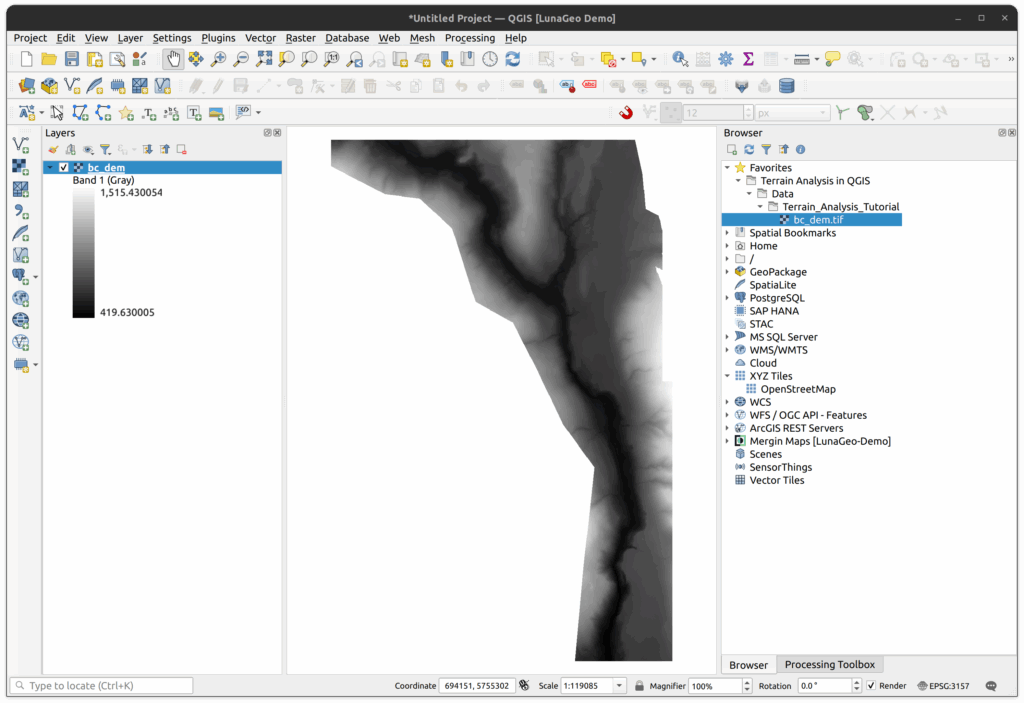
- Add the raster bc_dem.tif to the project. This is a digital elevation model (DEM). Cell values represent the elevation at that location. The light areas have high elevations and the dark areas have low elevations. Use the identify tool to examine the DEM.
- Open the layer properties and examine the Information and Source data.
- What is the CRS?
- What is the spatial resolution (pixel size)?
- How many bands are in the raster?
- In the symbology tab, what are the min and max values?
- Note you can change the Min / Max value setting, such as the accuracy can be switched from Estimate (faster) to Actual (slower).
- In the layer properties, under Symbology > Min/Max Value settings:
- Set to Min/Max.
- Set Statistics extent to the whole raster.
- Set Accuracy to Actual (slower).
- Click Apply and note that the min/max values change to the actual values.
- Close the layer properties.
- Save your project as bc_dem_terrain_analysis.qgz in the exercise directory.
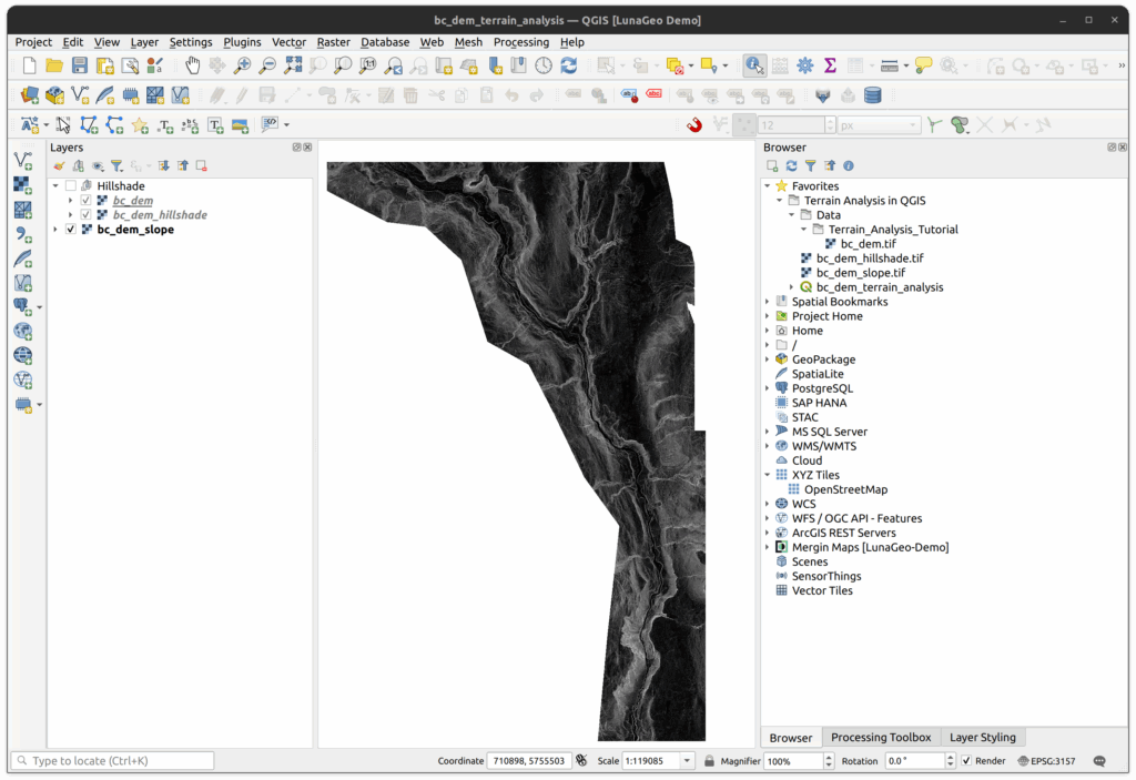
2. Create a Hillshade
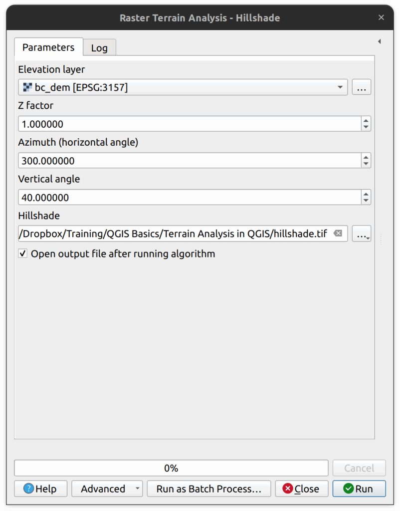
- We will first create a hillshade. Locate and open the Hillshade tool in the Processing panel.
- In the Hillshade tool, set the following parameters:
- Elevation layer is bc_dem.tif
- Z factor is 1.
- Azimuth (horizontal angle) can be left as 300 or you can experiment with this value.
- Vertical angle can be left as default (40).
- Save the hillshade as bc_dem_hillshade.tif in the tutorial directory.
- Click Run then Close when complete.
- The resulting hillshade should load automatically.
- You should now have two layers loaded into your QGIS project.
- Save the project.
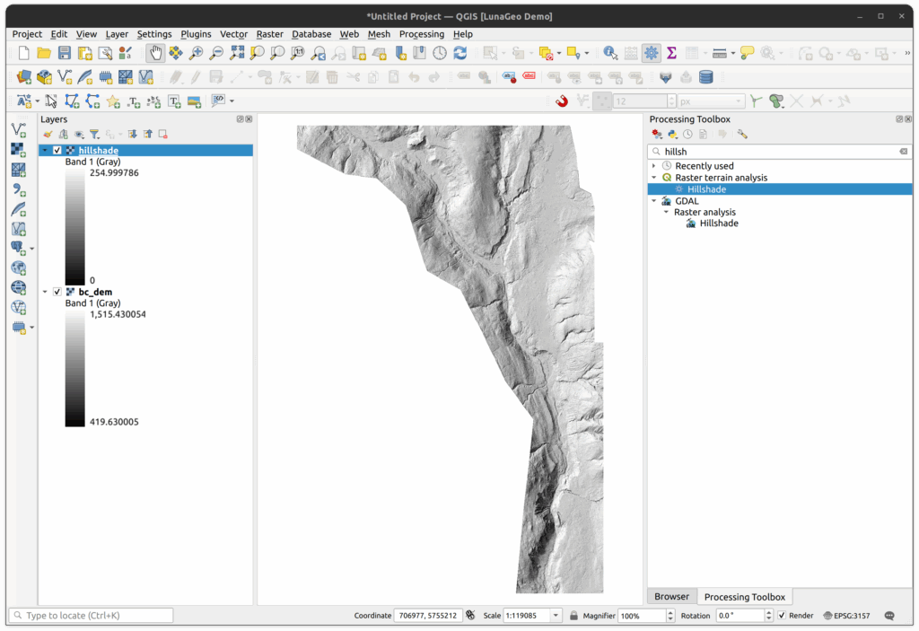
3. Style the Hillshade and DEM
- In the Layers panel, place the hillshade below the DEM layer.
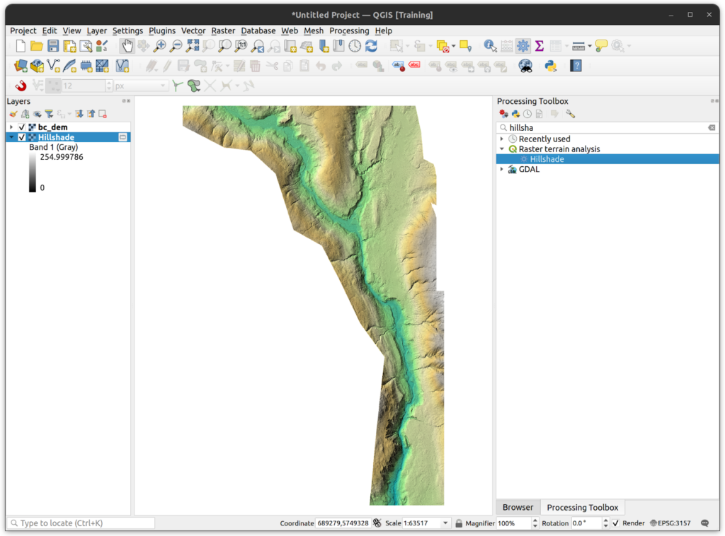
- Select the DEM layer and open the Layer Styling Panel.
- Switch to the Single Band Pseudocolor renderer.
- Click the colour ramp dropdown and select Create New Color Ramp…
- In the color ramp type window, select cpt-city and click OK.
- In the cpt-city Color Ramp window, select the Topography category.
- Select cd-a or sd-a (your choice) and click OK.
- Press Classify to apply the full range of the colour ramp to the raster.
- Scroll down to the Layer Rendering section and set the Blending mode to Multiply.
- Select both rasters in the Layers panel, then right click the selection and group the DEM and the hillshade. Call the group Hillshade. Turn the group visibility off.
- Save the project.
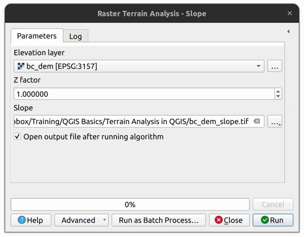
4. Calculate Slope
Next we will calculate the slope of the DEM in degrees.
- In the Processing Panel, expand the Raster Terrain Analysis group and double click on the Slope tool.
- Enter the following parameters:
- For the Elevation Layer, enter the bc_dem.tif
- Save the slope as bc_dem_slope.tif
- Click Run then close the tool to view the results. If the map remains blank after the tool completes, make sure the new slope raster is not in the Hillshade group in the Layers Panel. Right-click and select Move Out of Group.
- Use the identify tool to explore the slope layer.
- Open the layer properties to view the metadata.
- Run the Raster Layer Statistics tool on the slope layer to produce basic statistics for the layer. The results can be saved to the tutorial folder.
- We will reclassify this layer in Step 6 of this tutorial.
- Save the QGIS project.
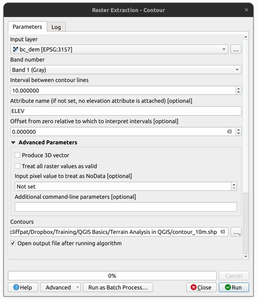
5. Create Contour Lines
5.1 Produce 10m Contours
- Next we will produce 10m contour lines using the BC DEM as the input layer.
- Locate and open the Contour tool in the Processing Panel.
- Set the following parameters:
- Set the input as bc_dem_tif (which should still be in your project even if it is not visible).
- Set the Interval to 10, which is 10m.
- Set the Attribute Name as ELEV
- Save the resulting vector layer into the tutorial folder. Name it contour_10m.shp.
- Click Run and Close when the process is complete. It will take a few seconds to run.
- Examine the contour lines. Toggle layers on/off if needed.
- You will notice that some of the contour as jagged and some are very small. Let’s clean up this dataset.
- Save the QGIS project.
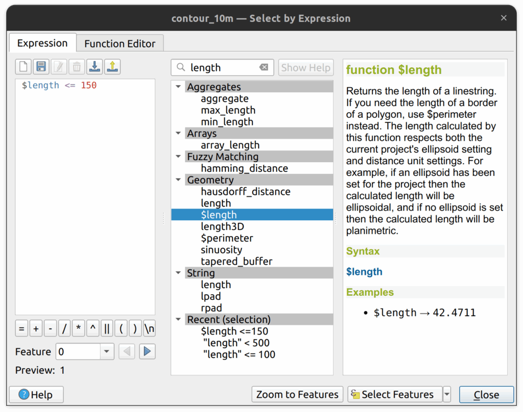
5.2 Delete Contours <= 150m in length
- To select all contours that are less than or equal to 150m in length, open the Select by Expression tool.
- Use the following expression: $length <= 150
- Look at the map canvas and note that all the smaller contours are selected. If you are happy with the selection, proceed to delete the selected features.
- Toggle editing to on and delete the selected features either from the Attributes table or by clicking the red garbage can icon on the editing toolbar.
- Toggle editing off and save changes when prompted to do so.
- Save the QGIS project.
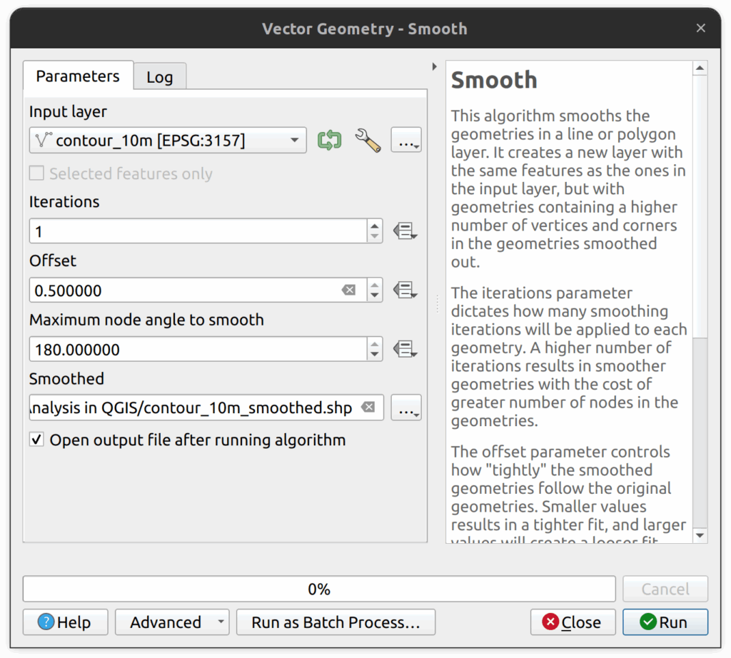
5.3 Smooth the contour lines
- Locate and open the Smooth tool in the Processing Panel.
- In the Smooth tool, set the following parameters:
- Iterations is 1.
- Offset is 0.5
- Maximum node angle to smooth is 180.
- Save the result as bc_dem_contours_smoothed.shp
- Click Run and Close when complete.
- The smoothed contours should look a lot neater. Examine and compare the two layers.
- Save the QGIS project.
6. Reclassify Slope Raster
1. Next we will reclassify the slope DEM to high and low slopes. We will define high slopes as 10 degrees to 90 degrees. Low slopes will be defined as anything less than or equal to 10 degrees.
2. Locate and open the tool called Reclassify by Table tool in the Processing panel.
3. In the Reclassify by Table tool, set the Raster layer as the slope layer (NOT the DEM).
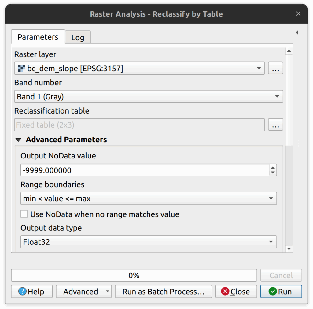
4. Select the Reclassification table button. In the reclassification table, add a row with min value of 0, max of 10 and give it the value 1. Then add another row and give it a min value of 10, max of 90 and value of 2. Click OK to return to the main tool settings.
5. Save the tool output as classified_slope.tif in the tutorial directory.
6. Click Run and then Close when it is complete.
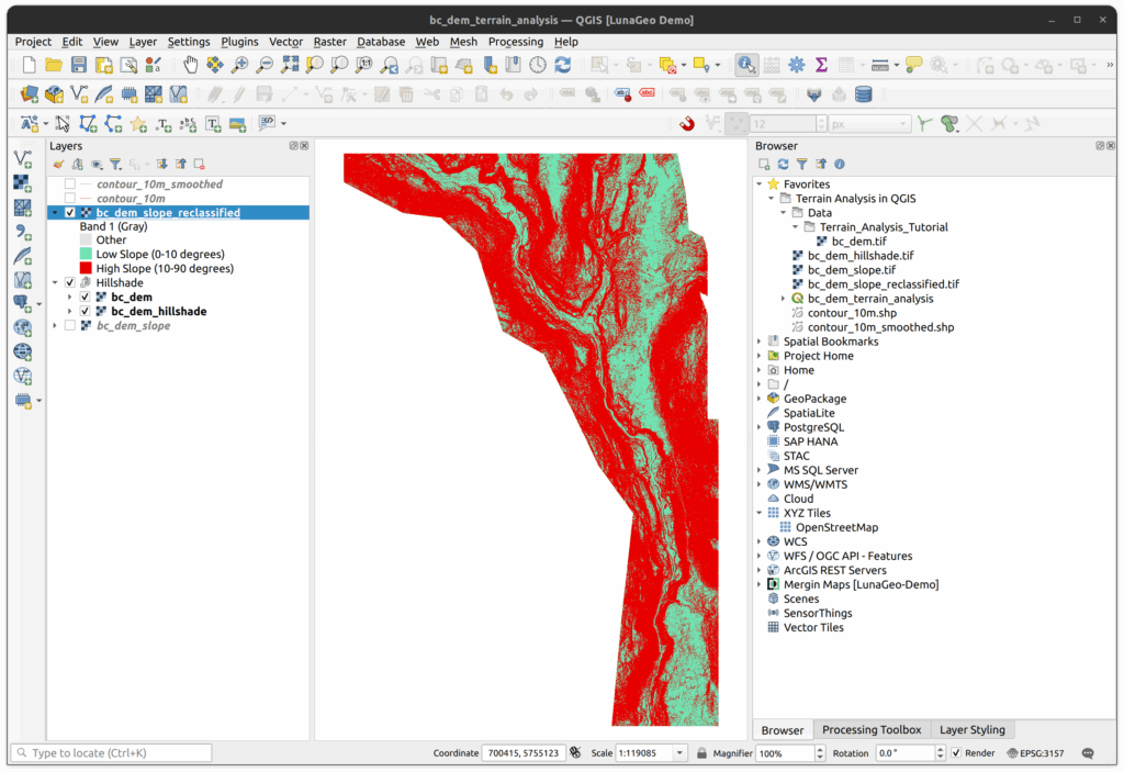
7. On the new raster layer, open the layer properties and change the symbology to the following:
- Change the render type to Paletted/Unique Values.
- Click Classify.
- Change the label for 0 values to “Other”.
- Change the label for 1 values to “Low Slope (0-10 degrees)”.
- Change the label for 2 values to “High Slope (10-90 degrees)”.
- Click OK.
You should now see a classified slope raster showing the relatively flat and higher slope areas.

How can we help?
Contact us today to schedule a free consultation with a member of our team.